5 Health Services and Policy Applications
5.1 Patient Satisfaction survey
In this chapter, we reproduce the analyses reported in the manuscript available at https://doi.org/10.1186/s12913-025-12596-x .
The first step in any empirical analysis is data acquisition. For this exercise, the dataset was imported into R using an R Markdown workflow. The Excel file (.xlsx), named DatasetNew, was stored on the desktop within a folder labeled Datasets and was read using the readxl package.
After importing the data, its structure was examined. The dataset contains 1,260 observations (rows) and 23 variables (columns).
library(readxl)
library(dplyr) # Must load dplyr to use select()

DatasetNew <- read_excel("/Users/corneille/Desktop/Datasets/DatasetNew.xlsx")
## New names:
## • `` -> `...3`# Exclude the unwanted column named '...4'
DatasetNew <- DatasetNew %>%
select(-`...3`)
#Explore number of rows and # columns
dim(DatasetNew)## [1] 1260 23## tibble [1,260 × 23] (S3: tbl_df/tbl/data.frame)
## $ No : num [1:1260] 1057 50 824 225 935 ...
## $ Province : chr [1:1260] "Eastern" "Kigali City" "Southern" "Eastern" ...
## $ District : chr [1:1260] "Nyagatare" "Kicukiro" "Muhanga" "Ngoma" ...
## $ Hospital : chr [1:1260] "Nyagatare DH" "Masaka DH" "Kabgayi Dh" "Kibungo RH" ...
## $ Age : num [1:1260] 36 58 46 54 80 28 33 41 22 39 ...
## $ Number of visits this year: num [1:1260] 1 2 2 3 3 1 1 1 1 1 ...
## $ visits : chr [1:1260] "new" "returning" "returning" "returning" ...
## $ AgeCategory : chr [1:1260] "Adult" "Adult" "Adult" "Adult" ...
## $ Hospitalgrp : chr [1:1260] "District" "District" "higherRanked" "higherRanked" ...
## $ location : chr [1:1260] "urban" "urban" "rural" "rural" ...
## $ Gender : chr [1:1260] "Female" "Female" "Female" "Female" ...
## $ entrance : chr [1:1260] "Yes" "Yes" "Yes" "Yes" ...
## $ reception : chr [1:1260] "Yes" "NA" "NA" "NA" ...
## $ cashier : chr [1:1260] "Yes" "Yes" "No" "Yes" ...
## $ waiting : chr [1:1260] "Yes" "Yes" "Yes" "No" ...
## $ triage : chr [1:1260] "Yes" "Yes" "Yes" "NA" ...
## $ medical doctor : chr [1:1260] "Yes" "Yes" "Yes" "Yes" ...
## $ confidentiality : chr [1:1260] "Yes" "Yes" "Yes" "Yes" ...
## $ asked the consent? : chr [1:1260] "No" "Yes" "No" "Yes" ...
## $ laboratory : chr [1:1260] "NA" "NA" "NA" "NA" ...
## $ dispensing pharmacy : chr [1:1260] "Yes" "Yes" "No" "Yes" ...
## $ radiolohgy : chr [1:1260] "NA" "NA" "NA" "NA" ...
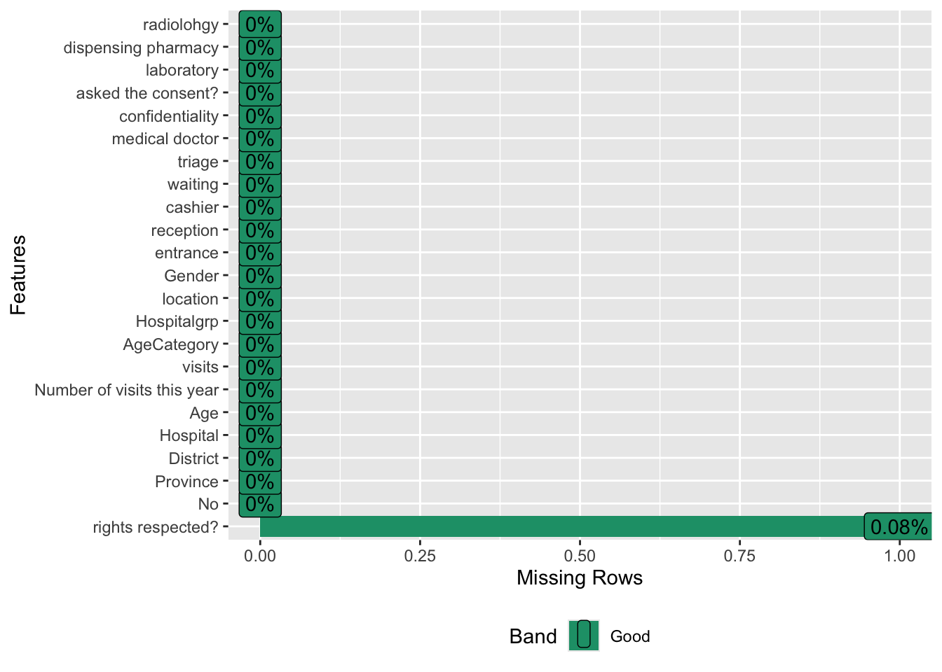
## $ rights respected? : chr [1:1260] "NA" "Yes" "Yes" "Yes" ...The second step is to check data quality. Here, I evaluated the percent of missingness for each variable.
Next, I created a new data frame restricted to complete cases, retaining only observations with no missing values in the specified variables.
# Load necessary packages
library(dplyr)
library(tidyr)

# 1. Define the set of variables to keep and check for completeness
varset <-

 c(

 'Province', 'visits', 'AgeCategory',
'Hospitalgrp', 'location', 'Gender', 'entrance', 'triage', 'medical doctor', 'laboratory', 'dispensing pharmacy', 'radiolohgy','rights respected?', 'waiting' , 'cashier'

 )

library(dplyr)

analytic.data <- DatasetNew %>%
  select(all_of(varset)) %>%      # keep only the variables in varset
  filter(complete.cases(.))       # keep only complete cases

dim(analytic.data)
## [1] 1259 15Prior to regression modeling, data harmonization was performed to ensure consistency and comparability across variables. This included recoding categorical variables, aligning variable formats, and verifying reference categories, thereby ensuring that all variables were appropriately structured for regression analysis.
#Recode Yes/No to 1/0

yes_no_vars <- c(
  "entrance",
  "triage",
  "medical doctor",
  "laboratory",
  "dispensing pharmacy",
  "radiolohgy",
  "rights respected?",
  "waiting",
  "cashier"
)

analytic.data <- analytic.data %>%
  mutate(across(all_of(yes_no_vars),
                ~ case_when(
                  . == "Yes" ~ 1,
                  . == "No"  ~ 0,
                  TRUE       ~ NA_real_
                )))

analytic.data <- analytic.data %>%
  mutate(
    Province = recode(Province,
                      "Eastern"      = 1,
                      "Kigali City"  = 2,
                      "Northern"     = 3,
                      "Southern"     = 4,
                      "Western"      = 5) |> as.numeric()
  )

analytic.data <- analytic.data %>%
  mutate(
    visits = recode(visits,
                    "new"        = 1,
                    "returning" = 2) |> as.numeric()
  )

analytic.data <- analytic.data %>%
  mutate(
    AgeCategory = recode(AgeCategory,
                         "young" = 1,
                         "Adult" = 2) |> as.numeric()
  )


analytic.data <- analytic.data %>%
  mutate(
    Hospitalgrp = recode(Hospitalgrp,
                         "District"     = 1,
                         "higherRanked" = 2) |> as.numeric()
  )

analytic.data <- analytic.data %>%
  mutate(
    location = recode(location,
                      "rural" = 1,
                      "urban" = 2) |> as.numeric()
  )

analytic.data <- analytic.data %>%
  mutate(
    Gender = recode(Gender,
                    "Male"   = 1,
                    "Female" = 2) |> as.numeric()
  )
Regression Analysis
The primary independent variable included in the regression model was location, which was specified according to the predefined categories in the dataset.
###location#

#crude analysis

MOD1 <- glm(waiting ~ location, family = "binomial", data = analytic.data)
summary(MOD1)
##
## Call:
## glm(formula = waiting ~ location, family = "binomial", data = analytic.data)
##
## Coefficients:
## Estimate Std. Error z value Pr(>|z|)
## (Intercept) 2.2377 0.2402 9.315 <2e-16 ***
## location -0.3619 0.1670 -2.168 0.0302 *
## ---
## Signif. codes: 0 '***' 0.001 '**' 0.01 '*' 0.05 '.' 0.1 ' ' 1
##
## (Dispersion parameter for binomial family taken to be 1)
##
## Null deviance: 1044.6 on 1249 degrees of freedom
## Residual deviance: 1040.0 on 1248 degrees of freedom
## (9 observations deleted due to missingness)
## AIC: 1044
##
## Number of Fisher Scoring iterations: 4## (Intercept) location
## 9.3718691 0.6963245## Waiting for profiling to be done...## 2.5 % 97.5 %
## (Intercept) 5.873786 15.0782390
## location 0.503278 0.9693642